Better registration of source –
The study of waves can be traced back to antiquity where philosophers, such as Pythagoras (c. 560-480 BC), studied the relation of pitch and length of string in musical instruments. However, it was not until the work of Giovani Benedetti (1530-90), Isaac Beeckman (1588-1637) and Galileo (1564-1642) that the relationship between pitch and frequency was discovered. This started the science of acoustics, a term coined by Joseph Sauveur (1653-1716) who showed that strings can vibrate simultaneously at a fundamental frequency and at integral multiples that he called harmonics. Isaac Newton (1642-1727) was the first to calculate the speed of sound in his Principia. However, he assumed isothermal conditions so his value was too low compared with measured values. This discrepancy was resolved by Laplace (1749-1827) when he included adiabatic heating and cooling effects. The first analytical solution for a vibrating string was given by Brook Taylor (1685-1731). After this, advances were made by Daniel Bernoulli (1700-82), Leonard Euler (1707-83) and Jean d’Alembert (1717-83) who found the first solution to the linear wave equation, see section (The linear wave equation). Whilst others had shown that a wave can be represented as a sum of simple harmonic oscillations, it was Joseph Fourier (1768-1830) who conjectured that arbitrary functions can be represented by the superposition of an infinite sum of sines and cosines – now known as the Fourier series. However, whilst his conjecture was controversial and not widely accepted at the time, Dirichlet subsequently provided a proof, in 1828, that all functions satisfying Dirichlet’s conditions (i.e. non-pathological piecewise continuous) could be represented by a convergent Fourier series. Finally, the subject of classical acoustics was laid down and presented as a coherent whole by John William Strutt (Lord Rayleigh, 1832-1901) in his treatise Theory of Sound. The science of modern acoustics has now moved into such diverse areas as sonar, auditoria, electronic amplifiers, etc.
The study of hydrostatics and hydrodynamics was being pursued in parallel with the study of acoustics. Everyone is familiar with Archimedes (c. 287-212 BC) eureka moment; however he also discovered many principles of hydrostatics and can be considered to be the father of this subject. The theory of fluids in motion began in the 17th century with the help of practical experiments of flow from reservoirs and aqueducts, most notably by Galileo’s student Benedetto Castelli. Newton also made contributions in the Principia with regard to resistance to motion, also that the minimum cross-section of a stream issuing from a hole in a reservoir is reached just outside the wall (the vena contracta). Rapid developments using advanced calculus methods by Siméon-Denis Poisson (1781-1840), Claude Louis Marie Henri Navier (1785-1836), Augustin Louis Cauchy (1789-1857), Sir George Gabriel Stokes (1819-1903), Sir George Biddell Airy (1801-92), and others established a rigorous basis for hydrodynamics, including vortices and water waves, see section (Physical wave types). This subject now goes under the name of fluid dynamics and has many branches such as multi-phase flow, turbulent flow, inviscid flow, aerodynamics, meteorology, etc.
The study of electromagnetism was again started in antiquity, but very few advances were made until a proper scientific basis was finally initiated by William Gilbert (1544-1603) in his De Magnete. However, it was only late in the 18th century that real progress was achieved when Franz Ulrich Theodor Aepinus (1724-1802), Henry Cavendish (1731-1810), Charles-Augustin de Coulomb (1736-1806) and Alessandro Volta (1745-1827) introduced the concepts of charge, capacity and potential. Additional discoveries by Hans Christian Ørsted (1777-1851), André-Marie Ampère (1775-1836) and Michael Faraday (1791-1867) found the connection between electricity and magnetism and a full unified theory in rigorous mathematical terms was finally set out by James Clerk Maxwell (1831-79) in his Treatise on Electricity and Magnetism. It was in this work that all electromagnetic phenomena and all optical phenomena were first accounted for, including waves, see section (Electromagnetic wave). It also included the first theoretical prediction for the speed of light.
At the end of the 19th century, when some erroneously considered physics to be very nearly complete, new physical phenomena began to be observed that could not be explained. These demanded a whole new set of theories that ultimately led to the discovery of general relativity and quantum mechanics; which, even now in the 21st century are still yielding exciting new discoveries. However, as this article is primarily concerned with classical wave phenomena, we will not pursue these topics further.
Historic data source: ‘Dictionary of The History of Science [Byn-84].
Introduction
A wave is a time evolution phenomenon that we generally model mathematically using partial differential equations (PDEs) which have a dependent variable u(x,t) (representing the wave value), an independent variable time t and one or more independent spatial variables x∈ℝn , where n is generally equal to 1,2or3 . The actual form that the wave takes is strongly dependent upon the system initial conditions, the boundary conditions on the solution domain and any system disturbances.
Waves occur in most scientific and engineering disciplines, for example: fluid mechanics, optics, electromagnetism, solid mechanics, structural mechanics, quantum mechanics, etc. The waves for all these applications are described by solutions to either linear or nonlinear PDEs. We do not focus here on methods of solution for each type of wave equation, but rather we concentrate on a small selection of relevant topics. However, first, it is legitimate to ask: what actually is a wave? This is not a straight forward question to answer.
Now, whilst most people have a general notion of what a wave is, based on their everyday experience, it is not easy to formulate a definition that will satisfy everyone engaged in or interested in this wide ranging subject. In fact, many technical works related to waves eschew a formal definition altogether and introduce the concept by a series of examples; for example, Physics of waves [Elm-69] and Hydrodynamics [Lam-93]. Nevertheless, it is useful to at least make an attempt and a selection of various definitions from normally authoritative sources is given below:
- “A time-varying quantity which is also a function of position” – Chambers Dictionary of Science and technology [Col-71].
- “… a wave is any recognizable signal that is transferred from one part of the medium to another with a recognizable velocity of propagation” – Linear and non-linear Waves [Whi-99].
- “Speaking generally, we may say that it denotes a process in which a particular state is continually handed on without change, or with only gradual change, from one part of a medium to another” – 1911 Encyclopædia Britannica.
- “a periodic motion or disturbance consisting of a series of many oscillations that propagate through a medium or space, as in the propagation of sound or light: the medium does not travel outward from the source with the wave but only vibrates as it passes” – Webster’s New World College Dictionary, 4th Ed.
- “… an oscillation that travels through a medium by transferring energy from one particle or point to another without causing any permanent displacement of the medium” – Encarta® World English Dictionary [Mic-07].
The variety of definitions given above, and their clearly differing degrees of clarity, confirm that ‘wave’ is indeed not an easy concept to define!
Because this is an introductory article and the subject of linear and non-linear waves is so wide ranging, we can only include sufficient material here to provide an overview of the phenomena and related issues. Relativistic issues will not be addressed. To this end we will discuss, as proxies for the wide range of known wave phenomena, the linear wave equation and the nonlinear Korteweg-de Vries equation in some detail by way of examples. To supplement this discussion we provide brief details of other types of wave equation and their application; and, finally, we introduce a number of PDE wave solution methods and discuss some general properties of waves. Where appropriate, references are included to works that provide further detailed discussion.
Physical wave types
A non-exhaustive list is given below of physical wave types with examples of occurrence and references where more details may be found.
- Acoustic waves – audible sound, medical applications of ultrasound, underwater sonar applications [Elm-69].
- Chemical waves – concentration variations of chemical species propagating in a system [Ros-88].
- Electromagnetic waves – electricity in various forms, radio waves, light waves in optic fibers, etc [Sha-75].
- Gravitational waves – The transmission of variations in a gravitational field in the form of waves, as predicted by Einstein’s theory of general relativity. Undisputed verification of their existence is still awaited [Oha-94, chapter 5].
- Seismic Waves – resulting from earthquakes in the form of P-waves and S-waves, large explosions, high velocity impacts [Elm-69].
- Traffic flow waves – small local changes in velocity occurring in high density situations can result in the propagation of waves and even shocks [Lev-07].
- Water waves – some examples
- Capillary waves (Ripples) – When ripples occur in water they are manifested as waves of short length, λ=2π/k<0.1m , (k=wavenumber) and in which surface tension has a significant effect. We will not consider them further, but a full explanation can be found in Lightfoot [Lig-78, p221]. See also Whitham [Whi-99, p404].
- Rossby (or planetary) waves – Long period waves formed as polar air moves toward the equator whilst tropical air moves to the poles – due to variation in the Coriolis effect. As a result of differences in solar radiation received at the equator and poles, heat tends to flow from low to high latitudes, and this is assisted by these air movements [Gil-82].
- Shallow water waves – For waves where the wavelength λ (distance between two corresponding points on the wave, e.g. peaks), is very much greater than water depth h , they can be modelled by the following simplified set of coupled fluid dynamics equations, known as the shallow water equations
⎡⎣⎢⎢⎢⎢∂h∂t∂u∂t⎤⎦⎥⎥⎥⎥+⎡⎣⎢⎢⎢⎢⎢∂(hu)∂x∂(12u2+gh)∂x⎤⎦⎥⎥⎥⎥⎥=⎡⎣⎢⎢⎢0−g∂b∂x⎤⎦⎥⎥⎥. (1)
-
- Where,
-
- b(x) = fluid bed topography
- h(x,t) = fluid surface height above bed
- u(x,t) = fluid velocity – horizontal
- g = acceleration due to gravity.
-
- For this situation, the celerity or speed of wave propagation can be approximated by c=gh‾‾‾√ . For detailed discussion refer to [Joh-97].
- Ship waves – These are surface waves that are formed by a ship travelling in deep water, relative to the wavelength, and where surface tension can be ignored. The dispersion relation is given by ω=gk‾‾√ ; so for phase velocity and group velocity see section (Group and phase velocity), we have respectively:
cp=ωk=gk‾‾√,(2)
cg=dω(k)dk=12cp. (3)
- The result is that the ship’s wake is a wedge-shaped envelope of waves having a semi-angle of ⋍19.5 degrees and a feathered pattern with the ship at the vertex. The shape is a characteristic of such waves, regardless of the size of disturbance – from a small duckling paddling on a pond to large ocean liner cruising across an ocean. These patterns are referred to as Kelvin Ship Waves after Lord Kelvin (William Thomson) [Joh-97].
-
- Tsunami waves – See section (Tsunami).
Linear waves
General
Linear waves are described by linear equations, i.e. those where in each term of the equation the dependent variable and its derivatives are at most first degree (raised to the first power).
This means that the superposition principle applies, and linear combinations of simple solutions can be used to form more complex solutions. Thus, all the linear system analysis tools are available to the analyst, with Fourier analysis: expressing general solutions in terms of sums or integrals of well known basic solutions, being one of the most useful. The classic linear wave is discussed in section (The linear wave equation) with some further examples given in section (Linear wave equation examples). Linear waves are modelled by PDEs that are linear in the dependent variable, u , and its first and higher derivatives, if they exist.
The linear wave equation
The following represents the classical wave equation in one dimension and describes undamped linear waves in an isotropic medium
1c2∂2u∂t2=∂2u∂x2.(4)
It is second order in t and x , and therefore requires two initial condition functions (ICs) and two boundary condition functions (BCs). For example, we could specify
ICs:u(x,t=0)=f(x),ut(x,t=0)=g(x),(5)
BCs:u(x=a,t)=ua,u(x=b,t)=ub.(6)
Consequently, equations (4), (5) and (6) constitute a complete description of the PDE problem.
We assume f to have a continuous second derivative (written f∈C2) and g to have a continuous first derivative (g∈C1). If this is the case, then u will have continuous second derivatives in x and t , i.e. (u∈C2), and will be a correct solution to equation (4) with any consistent set of appropriate ICs and BCs [Stra-92].
Extending equation (4) to three dimensions, the classical wave equation becomes,
1c2∂2u∂t2=∇2u,(7)
where ∇2=∇⋅∇ represents the Laplacian operator. Because the Laplacian is co-ordinate free, it can be applied within any co-ordinate system and for any number of dimensions. Given below are examples of wave equations in 3 dimensions for Cartesian, cylindrical and spherical co-ordinate systems
Cartesian co-ordinates:Cylindrical co-ordinates:Spherical co-ordinates:1c2∂2u∂t21c2∂2u∂t21c2∂2u∂t2===∂2u∂x2+∂2u∂y2+∂2u∂z2,1r∂∂r(r∂u∂r)+1r2∂2u∂θ2+∂2u∂z2,1r2∂∂r(r2∂u∂r)+1r2sinθ∂∂θ(sinθ∂u∂θ)+1r2sin2θ∂2u∂ϕ2.
These equations occur in one form or another, in numerous applications in all areas of the physical sciences; see for example section (Linear wave equation examples ).
The d’Alembert solution
The solution to equations (4), (5) and (6) was first reported by the French mathematician Jean-le-Rond d’Alembert (1717-1783) in 1747 in a treatise on Vibrating Strings [Caj-61] [Far-93]. D’Alembert’s remarkable solution, which used a method specific to the wave equation (based on the chain rule for differentiation), is given below
u(x,t)=12[f(x−ct)+f(x+ct)]+12c∫x+ctx−ctg(ξ)dξ.(8)
It can also be obtained by the Fourier Transform method or by the separation of variables (SOV) method, which are more general than the the method used by d’Alembert [Krey-93].
The d’Alembertian ◻=∇2−1c2∂2∂t2 , also known as the d’Alembert operator or wave operator, allows a succinct notation for the wave equation, i.e. ◻u=0 . It first arose in d’Alembert’s work on vibrating strings and plays a useful role in modern theoretical physics.
Linear wave equation examples
Acoustic (sound) wave
We will consider the acoustic or sound wave as a small amplitude disturbance of ambient conditions where second order effects can be ignored. We start with the Euler continuity and momentum equations
∂ρ∂t+∇⋅(ρv)=0,(9)
∂(ρv)∂t+∇⋅(ρvv)−ρg+∇p+∇⋅T=0,(10)
where
-
- T = stress tensor (Pa)
- g = gravitational acceleration (m/s2)
- p = pressure (Pa)
- t = time (s)
- v = fluid velocity (m/s)
- ρ = fluid density (kg/m3)
We assume an inviscid dry gas situation where gravitational effects are negligible. This means that the third and fifth terms of equation (10) can be ignored. If we also assume that we can represent velocity by v=u0+u , where uo is ambient velocity which we set to zero and u represents a small velocity disturbance, the second term in equation (10) can be ignored (because it becomes a second order effect). Thus, equations (9) and (10) reduce to
∂ρ∂t+∇⋅(ρu)=0,(11)
∂(ρu)∂t+∇p=0.(12)
Now, taking the divergence of equation (12) and the time derivative of equation (11), we obtain
∂2ρ∂t2−∇2p=0.
To complete the analysis we need to apply an equation-of-state relating p and ρ when we obtain the linear acoustic wave equation
1c2∂2p∂t2=∇2p,(13)
where
c2=∂p∂ρ .(14)
We now consider three cases:
- The isothermal gas case
p=ρRT0/MW
(ideal gas law) ⇒(∂p∂ρ)T=RT0/MW and c=RT0/MW‾‾‾‾‾‾‾‾‾√ , where T0 is the ambient temperature of the fluid, R is the ideal gas constant, MW is molecular weight and subscript T denotes constant temperature conditions.
- The isentropic gas case
p/ργ=K⇒(∂p∂ρ)s=γKργ−1=γRT0/MW
and c=γRT0/MW‾‾‾‾‾‾‾‾‾‾√ , where γ is the isentropic or adiabatic exponent for the fluid (equal to the ratio of specific heats) and subscript s denotes constant entropy conditions.
- The isothermal liquid case
(∂p∂ρ)T=β/ρ
and c=β/ρ‾‾‾√, where β is bulk modulus.
For atmospheric air at standard conditions we have p=101325Pa, T0=293.15K, R=8.3145J/mol/K, γ=1.4 and MW=0.028965kg/mol, which gives
isothermal:c=290m/s,(15)
isentropic:c=343m/s.(16)
For liquid distilled water at 20C we have β=2.18×10⁹Pa and ρ=1,000kg/m3, which gives
liquid:c=1476m/s.(17)
Waves in solids
Waves in solids are more complex than acoustic waves in fluids. Here we are dealing with displacement ϱ , and the resulting waves can be either longitudinal, P-waves, or shear (transverse), S-waves. Starting with Newton’s second Law we arrive at the vector wave equation [Elm-69, chapter 7]
(λ+μ)∇(∇⋅ϱ)+μ∇2ϱ=ρ∂2ϱ∂t2,(18)
from which, using the fundamental identity from vector calculus, ∇×(∇×ϱ)=∇(∇⋅ϱ)−∇2ϱ , we obtain
(λ+2μ)∇(∇⋅ϱ)+μ∇×(∇×ϱ)=ρ∂2ϱ∂t2.(19)
Now, for irrotational waves, which vibrate only in the direction of propagation x , ∇×ϱ=0⇒∇(∇⋅ϱ)=∇2ϱ and equation (19) reduces to the familiar linear wave equation
1c2∂2ϱ∂t2=∇2ϱ,(20)
where c=(λ+2μ)/ρ‾‾‾‾‾‾‾‾‾‾√=(K+43μ)/ρ‾‾‾‾‾‾‾‾‾‾‾‾√ is the wave speed, λ=Eυ/(1+υ)(1−2υ) is the Lamé modulus, μ=E2(1+υ) is the shear modulus and K=E/3(1−2υ) is the bulk modulus of the solid material. Here, E and υ are Young’s modulus and Poisson’s ratio for the solid respectively. Irrotational waves are of the longitudinal type, or P-waves.
For solenoidal waves, which can vibrate independently in the y and z directions but not in the direction of propagation x , we have ∇⋅ϱ=0 and equation (18) reduces to the linear wave equation
1c2∂2ϱ∂t2=∇2ϱ,(21)
where the wave speed is given by c=μ/ρ‾‾‾√ . Solenoidal waves are of the transverse type, or S-waves.
For a typical mild-steel at 20C with ρ=7,860kg/m3 , E=210×109N/m2 and υ=0.29 we find that the P-wave speed is 5917m/s and the S-wave speed is 3,218m/s. For further discussion refer to [Cia-88].
Electromagnetic waves
The fundamental equations of electromagnetism are the Maxwell Equations, which in differential form and SI units, are usually written as:
∇⋅E=1ϵ0ρ,(22)
∇⋅B=0,(23)
∇×E=−∂B∂t,(24)
∇×B=μ0J+μ0ϵ0∂E∂t,(25)
where
-
- B= magnetic field (T)
- E= electric field (V/m)
- J= current density (A/m2)
- t= time (s)
- ϵ0= permittivity of free space (8.8541878×10⁻¹²≃10−9/36π F/m)
- μ0= permeability of free space (4π×10−7 H/m)
- ρ= charge density (C/m3)
If we assume that J=0 and ρ=0 , then on taking the curl of equation (24) and again using the fundamental identity from vector calculus, ∇×(∇×E)=∇(∇⋅E)−∇2E , we obtain
1c20∂2E∂t2=∇2E.(26)
Similarly, taking the curl of equation (25) we obtain
1c20∂2B∂t2=∇2B.(27)
Equations (26) and (27) are the linear electric and magnetic wave equations respectively, where c0=1/μ0ϵ0‾‾‾‾√≃3×108 m/s, the speed of light in a vacuum. They take the familiar form of linear wave equation (4). For further discussion refer to [Sha-75].
Nonlinear waves
General
Nonlinear waves are described by nonlinear equations, and therefore the superposition principle does not generally apply. This means that nonlinear wave equations are more difficult to analyze mathematically and that no general analytical method for their solution exists. Thus, unfortunately, each particular wave equation has to be treated individually. An example of solving the Korteweg-de Vries equation by direct integration is given below.
Some advanced methods that have been used successfully to obtain closed-form solutions are listed in section (Closed form PDE solution methods), and example solutions to well known evolution equations are given in section (Nonlinear wave equation solutions).
Closed form PDE solution methods
There are no general methods guaranteed to find closed form solutions to non-linear PDEs. Nevertheless, some problems can yield to a trial-and-error approach. This hit-and-miss method seeks to deduce candidate solutions by looking for clues from the equation form, and then systematically investigating whether or not they satisfy the particular PDE. If the form is close to one with an already known solution, this approach may yield useful results. However, success is problematical and relies on the analyst having a keen insight into the problem.
We list below, in alphabetical order, a non-exhaustive selection of advanced solution methods that can assist in determining closed form solutions to nonlinear wave equations. We will not discuss further these methods and refer the reader to the references given for details. All these methods are greatly enhanced by use of a symbolic computer program such as: Maple V, Mathematica, Macysma, etc.
- Bäcklund transformation – A method used to find solutions to a non-linear partial differential equation from either a known solution to the same equation or from a solution to another equation. This can facilitate finding more complex solutions from a simple solution, e.g. a multi-soliton solutions from a single soliton solution [Abl-91],[Inf-00],[Dra-89].
- Generalized separation of variables method – For simple cases this method involves searching for exact solutions of the multiplicative separable form u(x,t)=φ(x)ψ(t) or, of the additive separable form u(x,t)=φ(x)+ψ(t) , where φ(x) and ψ(t) are functions to be found. The chosen form is substituted into the original equation and, after performing some algebraic operations, two expressions are obtained that are each deemed equal to a constant K , the separation constant. Each expression is then solved independently and then combined additively or multiplicatively as appropriate. Initial conditions and boundary conditions are then applied to give a particular solution to the original equation. For more complex cases, special solution forms such as u(x,t)=φ(x)ψ(t)+χ(x) can be sought – refer to [Pol-04, pp. 698-712], [Gal-06], and [Pol-07, pp. 681-696] for a detailed discussion.
- Differential constraints method – This method seeks particular solutions of equations of the form F(x,y,u,∂u∂x,∂u∂y,∂2u∂x2,∂2u∂x∂y,∂2u∂y2,⋯)=0 by supplementing them with an additional differential constraint(s) of the form G(x,y,u,∂u∂x,∂u∂y,∂2u∂x2,∂2u∂x∂y,∂2u∂y2,⋯)=0 . The exact form of the differential constraint is determined from auxiliary problem conditions, usually based on physical insight. Compatibility analysis is then performed, for example by differentiating F and G (possibly several times), which enables an ordinary differential equation(s) to be constructed that can be solved. The resulting ODE is the compatibility condition for F and G and its solution can be used to obtain a solution to the original equation – refer to [Pol-04, pp. 747-758] for a detailed discussion.
- Group analysis methods (Lie group methods) – These methods seeks to identify symmetries of an equation which permit us to discover: (i) transformations under which the equation is invariant, (ii) new variables in which the structure of the equation is simplified. For an (n+1)-dimensional Euclidean space, the set of transformations Tϵ={xi¯=φi(x,u,ϵ),u¯=ψ(x,u,ϵ),xi¯∣∣ϵ=0=xiu¯∣∣ϵ=0=u , where φi and ψ are smooth functions of their arguments and ϵ is a real parameter, is called a one-parameter continuous point Lie group of transformations, G , if for all ϵ1 and ϵ2 we have Tϵ1∘Tϵ2=Tϵ1+ϵ2 – refer to [Ibr-94] and [Pol-04, pp. 735-743] for a detailed discussion.
- Hirota’s bilinear method – This method can be used to construct periodic and soliton wave solutions to nonlinear PDEs. It seeks a solution of the form u=−2(logf)xx by introducing the bilinear operator DmtDnx(a⋅b)=(∂∂t−∂∂t′)m(∂∂x−∂∂x′)na(x,t)b(x′,t′)∣∣∣x′=xt′=t for non-negative integers m and n [Joh-97],[Dai-06].
- Hodograph transformation method – This method belongs to the class of point transformations and involves the interchange of dependent and independent variables, i.e. τ=t , ξ=u(x,t) , η(ξ,τ)=x . This transformation can, for certain applications, result in a simpler (possibly an exact linearization) problem for which solutions can be found [Cla-89], [Pol-04, pp. 686-687].
- Inverse scattering transform (IST) method – The phenomenon of scattering refers to the evolution of a wave subject to certain conditions, such as boundary and/or initial conditions. If data relating to the scattered wave are known, then it may be possible to determine from these data the underlying scattering potential. The problem of reconstructing the potential from the scattering data is referred to as the so-called inverse scattering transform. The IST is a nonlinear analog of the Fourier transform used for solving linear problems. This useful property allows certain nonlinear problems to be treated by what are essentially linear methods. The IST method has been used for solving many types of evolution equation [Abl-91], [Inf-00], [Kar-98], [Whi-99].
- Lax pairs – A Lax pair consists of the Lax operator L (which is self-adjoint and may depend upon x,ux,uxx,⋯ , but not explicitly upon t) and the operator A that together represent a given partial differential equation such that Lt=[A,L]=(AL−LA) . Note
(AL−LA)
represents the commutator of the operators L and A . Operator A is required to have enough freedom in any unknown parameters or functions to enable the operator Lt=[L,A] to be chosen so that it is of degree zero, i.e. a multiplicative operator. L and A can be either scalar or matrix operators. If a suitable Lax pair can be found, the analysis of the nonlinear equation can be reduced to that of two simpler equations. However, the process of finding L and A corresponding to a given equation can be quite difficult. Therefore, if a clue(s) is available, inverting the process by first postulating a given L and A and then determining which partial differential equation they correspond to, can sometimes lead to good results. However, this may require the determination of many trial pairs and, ultimately, may not lead to the required solution [Abl-91],[Inf-00],[Joh-97],[Pol-07].
- Painlevé test – The Painlevé test is used as a means of predicting whether or not an equation is likely to be integrable. The test involves checking of self-similar reduced equations against a set of the six Panlevé equations (or, Panlevé transcendents) and, if there is a match, the system is integrable. A nonlinear evolution equation which is solvable by the IST is a Panelevé type, which means that it has no movable singularities other than poles [Abl-91],[Joh-97].
- Self-similar and similarity solutions – An example of a self-similar solution to a nonlinear PDE is a solution where knowledge of u(x,t=t0) is sufficient to obtain u(x,t) for all t>0 , by suitable rescaling [Bar-03]. In addition, by choosing a suitable similarity transformation(s) it is sometimes possible to find a similarity solution whereby a combination of variables is invariant under the similarity transformation [Fow-05].
Some techniques for obtaining traveling wave solutions
The following are examples of techniques that transform PDEs into ODEs which are subsequently solved to obtain traveling wave solutions to the original equations.
- Exp-function method – This is a straight forward method that assumes a traveling wave solution of the form u(x,t)=u(η) where η=kx+ωt , ω= frequency and k= wavenumber. This transforms the PDE into an ODE. The method then attempts to find solutions of the form u(η)=∑dn=−canexp(nη)∑qm=−pbmexp(mη) , where c , d , p and q are positive integers to be determined, and an and bm are unknown constants [He-06].
- Factorization – This method seeks solutions PDEs with a polynomial non-linearity by rescaling to eliminate coefficients and assuming a travelling wave solution of the form u(x,t)=U(ξ) , where ξ=k(x−vt) , v= velocity and k= wavenumber. The resulting ODE is then factorized and each factor solved independently [Cor-05].
- Tanh method – This is a very useful method that is conceptually easy to use and has produced some very good results. Basically, it assumes a travelling wave solution of the form u(x,t)=U(ξ) where ξ=k(x−vt) , v= velocity and k= wavenumber. This has the effect of transforming the PDE into a set of ODEs which are subsequently solved using the transformation Y=tanh(ξ) [Mal-92],[Mal-96a],[Mal-96b].
Some example applications of these and other methods can be found in [Gri-11].
Nonlinear wave equation solutions
A non-exhaustive selection of well known 1D nonlinear wave equations and their closed-form solutions is given below. The closed form solutions are given by way of example only, as nonlinear wave equations often have many possible solutions.
- Hopf equation (inviscid Burgers equation): ut+uux=0 [Pol-02]
-
- – Applications: gas dynamics and traffic flow.
- – Solution
u=φ(ξ),ξ=x−φ(ξ)t.
-
- where
-
- u(x,t=0)=φ(x), arbitrary initial condition.
- Burgers equation: ut+uux−auxx=0 [Her-05]
-
- – Applications: acoustic and hydrodynamic waves.
- – Solution
u(x,t)=2ak[1−tanhk(x−Vt)].
-
- where
-
-
-
- k= wavenumber,
- V=velocity,
- a= arbitrary constant.
-
- – Applications: heat and mass transfer, population dynamics, ecology.
- – Solution
u(x,t)=14{1−tanhk[x−Vt]}2.
-
- where
-
-
-
- k=126‾√ (wavenumber),
- V=56‾√ (velocity).
- Note: wavenumber and velocity are fixed values.
- Sine Gordon equation: utt=auxx+bsin(λu) [Pol-07]
-
- – Applications: various areas of physics
- – Solution
u(x,t)=⎧⎩⎨⎪⎪⎪⎪⎪⎪⎪⎪4λarctan⎡⎣⎢⎢⎢exp⎛⎝⎜⎜⎜±bλ(kx+μt+θ0)bλ(μ2−ak2)‾‾‾‾‾‾‾‾‾‾‾‾‾√⎞⎠⎟⎟⎟⎤⎦⎥⎥⎥,bλ(μ2−ak2)>0,4λarctan⎡⎣⎢⎢⎢exp⎛⎝⎜⎜⎜±bλ(kx+μt+θ0)bλ(ak2−μ2)‾‾‾‾‾‾‾‾‾‾‾‾‾√⎞⎠⎟⎟⎟⎤⎦⎥⎥⎥−πλ,bλ(μ2−ak2)<0.
-
- where
-
-
-
- k= wavenumber,
- μ,θ0= arbitrary constants.
- Cubic Schrödinger equation: iut+uxx+q∣∣u∣∣2u=0 [Whi-99]
-
- – Applications: various areas of physics, non-linear optics, superconductivity, plasma models.
- – Solution
u(x,t)=αq‾‾√sech(α‾‾√(x−Vt)),α>0,q>0.
-
- where
-
-
-
- V=velocity,
- α,q= arbitrary constants.
- Korteweg-de Vries (a variant)
ut+uux+buxxx=0
[Her-05]
-
- – Applications: various areas of physics, nonlinear mechanics, water waves.
- – Solution
u(x,t)=12bk2sech2k(x−Vt)
-
- where
-
-
-
- k=wavenumber,
- V=velocity,
- b= arbitrary constant.
- Boussinesq equation: utt−uxx+3uuxx+αuxxxx=0 [Abl-91]
-
- – Applications: surface water waves
- – Solution
16{1+8k2−V2}−2k2tanh2k(x+Vt)
-
- where
-
-
-
- k=wavenumber,
- V=velocity.
- Nonlinear wave equation of general form: utt=[f(u)ux]x
- This equation can be linearized in the general case. Some exact solutions are given in [Pol-04, pp252-255] and, by way of an example consider the following special case where f(u)=αeλu :
-
- Wave equation with exponential non-linearity: utt=(αeλuux)x,α>0. [Pol-04, p223]
- – Applications: traveling waves
- – Solution
u(x,t)=1λln(αax2+bx+c)−2λln(αat+d) :
-
- where
-
-
-
- α,λ,a,b,c,d= arbitrary constants.
Additional wide-ranging examples of traveling wave equations, with solutions, from the fields of mathematics, physics and engineering are given in Polyanin & Manzhirov [Pol-07] and Polyanin & Zaitsev [Pol-04]. Examples from the biological and medical fields can be found in Murray [Mur-02] and Murray [Mur-03]. A useful on-line resource is the DispersiveWiki [Dis-08].
The Korteweg-de Vries equation
The canonical form of the Korteweg-de Vries (KdV) equation is
∂u∂t−6u∂u∂x+∂3u∂x3=0,(28)
and is a non-dimensional version of the following equation originally derived by Korteweg and de Vries for a moving (Lagrangian) frame of reference [Jag-06], [Kor-95],
∂η∂τ=32gho‾‾‾√∂∂χ[12η2+23αη+13σ∂2η∂χ2].(29)
It is, historically, the most famous solitary wave equation and describes small amplitude, shallow water waves in a channel, where symbols have the following meaning:
-
- g= gravitational acceleration (m/s2)
- ho= nominal water depth (m)
- T= capillary surface tension of fluid (N/m)
- α= small arbitrary constant related to the uniform motion of the liquid (dimensionless)
- η= wave height (m)
- ρ= fluid density (kg/m3)
- τ= time (s)
- χ= distance (m)
After re-scaling and translating the dependent and independent variables to eliminate the physical constants using the transformations [Abl-91],
u=−12η−13α;x=−χσ‾‾√;t=12ghoσ‾‾‾‾‾√τ(30)
where σ=h3o/3−Tho/(ρg) , and Tho/(ρg) is called the Bond number (a measure of the relative strengths of surface tension and gravitational force), we arrive at the Korteweg-de Vries equation, i.e. equation (28).
The basic assumptions for the derivation of KdV waves in liquid, having wavelength λ , are [Abl-91]:
- the waves are long waves in comparison with total depth, hoλ≪1 ;
- the amplitude of the waves is small, ε=ηho≪1 ;
- the first two effects approximately balance, i.e. hoλ=(ε) ;
- viscous effects can be neglected.
The KdV equation was found to have solitary wave solutions [Lam-93], which confirmed John Scott-Russell’s account of the solitary wave phenomena [Sco-44] discovered during his experimental investigations into water flow in channels to determine the most efficient design for canal boats [Jag-06]. Subsequently, the KdV equation has been shown to model various other nonlinear wave phenomena found in the physical sciences. John Scott-Russell, a Scottish engineer and naval architect, also described in poetic terms his first encounter with the solitary wave phenomena, thus:
“I was observing the motion of a boat which was rapidly drawn along a narrow channel by a pair of horses, when the boat suddenly stopped – not so the mass of water in the channel which it had put in motion; it accumulated round the prow of the vessel in a state of violent agitation, then suddenly leaving it behind, rolled forward with great velocity, assuming the form of a large solitary elevation, a rounded, smooth and well-defined heap of water, which continued its course along the channel apparently without change of form or diminution of speed. I followed it on horseback, and overtook it still rolling on at a rate of some eight or nine miles an hour, preserving its original figure some thirty feet long and a foot to a foot and a half in height. Its height gradually diminished, and after a chase of one or two miles I lost it in the windings of the channel. Such, in the month of August 1834, was my first chance interview with that singular and beautiful phenomenon which I have called the Wave of Translation” [Sco-44].
An experimental apparatus for re-creating the phenomena observed by Scott-Russell have been built at Herriot-Watt University. Scott-Russell also coined the term solitary wave and conducted some of the first experiments to investigate another nonlinear wave phenomena, the Doppler effect, publishing an independent explanation of the theory in 1848 [Sco-48].
It is interesting to note that, a KdV solitary wave in water that experiences a change in depth will retain its general shape. However, on encountering shallower water its velocity and height will increase and its width decrease; whereas, on encountering deeper water its velocity and height will decrease and its width increase [Joh-97, pp 268-277].
A closed form single soliton solution to the KdV equation (28) can be found using direct integration as follows.
Assume a travelling wave solution of the form
u(x,t)=f(x−vt)=f(ξ).(31)
Then on substituting into the canonical equation the PDE is transformed into the following ODE
−vdf(ξ)dξ−6fdf(ξ)dξ+d3f(ξ)dξ3=0.(32)
Now integrate with respect to ξ and multiply by df(ξ)dξ to obtain
−vf(ξ)df(ξ)dξ−3f(ξ)2df(ξ)dξ+df(ξ)dξ(d2f(ξ)dξ2)=Adf(ξ)dξ.(33)
Now integrate with respect to ξ once more, to obtain
−12vf(ξ)2−f(ξ)3+12(df(ξ)dξ)2=Af(ξ)+B.(34)
Where A and B are arbitrary constants of integration which we set to zero. We justify this by assuming that we are modeling a physical system with properties such that f,f′ and f′′→0 as ξ→±∞ . After rearranging and evaluating the resulting integral, we find
f(ξ)=v2sech2(v√2ξ).(35)
The solution is therefore
u(x,t)=f(x−vt),(36)
=2k2sech2(k[x−vt−x0]),(37)
where k=v√2 represents wavenumber and the constant x0 has been included to locate the wave peak at t=0 . Thus, we observe that the wave travels to the right with a speed that is equal to twice the peak amplitude. Hence, the taller a wave the faster it travels.
The KdV equation also admits many other solutions including multiple soliton solutions, see figure (15), and cnoidal (periodic) solutions.
Solutions of KdV equation can be systematically obtained from solutions ψi of of the free particle Schrödinger equation
−(∂2∂x2ψi)=Eiψi,i=1,⋯,n(38)
using the the relationship
u(x,t)=2(∂2∂x2ln(Wn)),(39)
where we use the the Wronskian function
Wn=Wn[ψ1,ψ2,⋯,ψn].(40)
The Wronskian is the determinant of a n×n matrix [Dra-89] composed from the functions ψi(ξi) , where ξi for our purposes is given by
ξi=ki(x−vit),Ei<0,(41)
ξi=ki(x+vit),Ei>0.(42)
For example, a two-soliton solution is given by
u(x,t)=(k21−k22){2k22cschk2(x−v2t)+2k21sechk1(x−v1t)}[k1tanhk1(x−v1t)+k2cothk2(x−v2t)]2(43)
and a cnoidal wave solution is given by
u(x,t)=16k(4k2(2m−1)−vk)−2k2cn2(kx−vkt+x0;m).(44)
where ‘cn’ represents the Jacobi elliptic cosine function with modulus m,(0<m<1). Note: as m→1 the periodic solution tends to a single soliton solution.
Interestingly, the KdV equation is invariant under a Galilean transformation, i.e. its properties remain unchanged, see section (Galilean invariance).
Numerical solution methods
Linear and nonlinear evolutionary wave problems can very often be solved by application of general numerical techniques such as: finite difference, finite volume, finite element, spectral, least squares, weighted residual (e.g. collocation and Galerkin) methods, etc. These methods, which can all handle various boundary conditions, stiff problems and may involve explicit or implicit calculations, are well documented in the literature and will not be discussed further here. For general texts refer to [Bur-93],[Sch-94],[Sch-09], and for more detailed discussion refer to [Lev-02],[Mor-94],[Zie-77].
Some wave problems do, however, present significant problems when attempting to find a numerical solution. In particular we highlight problems that include shocks, sharp fronts or large gradients in their solutions. Because these problems often involve inviscid conditions (zero or vanishingly small viscosity), it is often only practical to obtain weak solutions. Some PDE problems do not have a mathematically rigorous solution, for example where discontinuities or jump conditions are present in the solution and/or characteristics intersect. Such problems are likely to occur when there is a hyperbolic (strongly convective) component present. In these situations weak solutions provide useful information. Detailed discussion of this approach is beyond the scope of this article and readers are referred to [Wes-01, chapters 9 and 10] for further discussion.
General methods are often not adequate for accurate resolution of steep gradient phenomena; they usually introduce non-physical effects such as smearing of the solution or spurious oscillations. Since publication of Godunov’s order barrier theorem, which proved that linear methods cannot provide non-oscillatory solutions higher than first order [God-54],[God-59], these difficulties have attracted a lot of attention and a number of techniques have been developed that largely overcome these problems. To avoid spurious or non-physical oscillations where shocks are present, schemes that exhibit a total variation diminishing (TVD) characteristic are especially attractive. Two techniques that are proving to be particularly effective are MUSCL (Monotone Upstream-Centred Schemes for Conservation Laws) a flux/slope limiter method [van-79],[Hir-90],[Tan-97],[Lan-98],[Tor-99] and the WENO (Weighted Essentially Non-Oscillatory) method [Shu-98],[Shu-09]. MUSCL methods are usually referred to as high resolution schemes and are generally second-order accurate in smooth regions (although they can be formulated for higher orders) and provide good resolution, monotonic solutions around discontinuities. They are straight-forward to implement and are computationally efficient. For problems comprising both shocks and complex smooth solution structure, WENO schemes can provide higher accuracy than second-order schemes along with good resolution around discontinuities. Most applications tend to use a fifth order accurate WENO scheme, whilst higher order schemes can be used where the problem demands improved accuracy in smooth regions.
Initial conditions and boundary conditions
Consider the classic 1D linear wave equation
∂2u∂t2=1c2∂2u∂x2.(45)
In order to obtain a solution we must first specify some auxiliary conditions to complete the statement of the PDE problem. The number of required auxiliary conditions is determined by the highest order derivative in each independent variable. Since equation (45) is second order in t and second order in x , it requires two auxiliary conditions in t and two auxiliary conditions in x . To have a complete well posed problem, some additional conditions may have to be included – refer to section (Wellposedness).
The variable t is termed an initial value variable and therefore requires two initial conditions (ICs). It is an initial value variable since it starts at an initial value, t0 , and moves forward over a finite interval t0≤t≤tf or a semi-infinite interval t0≤t≤∞ without any additional conditions being imposed. Typically in a PDE application, the initial value variable is time, as in the case of equation (45).
The variable x is termed a boundary value variable and therefore requires two boundary conditions (BCs). It is a boundary value variable since it varies over a finite interval x0≤x≤xf , a semi-infinite interval x0≤x≤∞ or a fully infinite interval −∞≤x≤∞ , and at two different values of x, conditions are imposed on u in equation (45). Typically, the two values of x correspond to boundaries of a physical system, and hence the name boundary conditions.
BCs can be of three types:
- Dirichlet or first type – the boundary has a value u(x=x0,t)=ub(t) .
- Neumann or second type – the spatial gradient at the boundary has a value ∂u(x=xf,t)∂x=ubx(t) , and for multi-dimensions it is normal to the boundary.
- Robin or third type – both the dependent variable and its spatial derivative appear in the BC, i.e. a combination of Dirichlet and Neumann.
An important consideration is the possibility of discontinuities at the boundaries, produced for example by differences in initial and boundary conditions at the boundaries, which can cause computational difficulties, such as shocks – see section (Shock waves), particularly for hyperbolic PDEs such as equation (45) above.
Numerical dissipation and dispersion
General
Some dissipation and dispersion occur naturally in most physical systems described by PDEs. Errors in magnitude are termed dissipation and errors in phase are called dispersion. These terms are defined below. The term amplification factor is used to represent the change in the magnitude of a solution over time. It can be calculated in either the time domain, by considering solution harmonics, or in the complex frequency domain by taking Fourier transforms.
Dissipation and dispersion can also be introduced when PDEs are discretized in the process of seeking a numerical solution. This introduces numerical errors. The accuracy of a discretization scheme can be determined by comparing the numeric amplification factor Gnumeric, with the analytical or exact amplification factor Gexact , over one time step.
For further reading refer to [Hir-88, chap. 8], [Lig-78, chap. 3], [Tan-97, chap. 4], [Wes-01, chap 8 and 9].
Dispersion relation
Physical waves that propagate in a particular medium will, in general, exhibit a specific group velocity as well as a specific phase velocity – see section (Group and phase velocity). This is because within a particular medium there is a fixed relationship between the wavenumber k , and the frequency ω , of waves. Thus, frequency and wavenumber are not independent quantities and are related by a functional relationship, known as the dispersion relation , ω(k).
We will demonstrate the process of obtaining the dispersion relation by example, using the advection equation
ut+aux=0.(46)
Generally, each wavenumber k , corresponds to s frequencies where s is the order of the PDE with respect to t . Now any linear PDE with constant coefficients admits a solution of the form
u(x,t)=u0ei(kx−ωt).(47)
Because we are considering a linear system, the principal of superposition applies and equation (47) can be considered to be a frequency component or harmonic of the Fourier series representation of a specific solution to the advection equation. On inserting this solution into a PDE we obtain the so called dispersion relation between ω and k i.e.,
ω=ω(k),(48)
and each PDE will have its own distinct form. For example, we obtain the specific dispersion relation for the advection equation by substituting equation (47) into equation (46) to get
−iωu0ei(kx−ωt)=−iaku0ei(kx−ωt)
⇓
ω=ak.(49)
This confirms that ω and k cannot be determined independently for the advection equation, and therefore equation (47) becomes
u(x,t)=u0eik(x−at).(50)
Note: If the imaginary part of ω(k) is zero, then the system is non-dissipative.
The physical meaning of equation (50) is that the initial value u(x,0)=u0eikx , is propagated from left to right, unchanged, at velocity a . Thus, there is no dissipation or attenuation and no dispersion.
A similar approach can be used to establish the dispersion relation for systems described by other forms of PDEs.
Amplification factor
As mentioned above, the accuracy of a numerical scheme can be determined by comparing the numeric amplification factor Gnumeric, with the exact amplification factor Gexact , over one time step. The exact amplification factor can be determined by considering the change that takes place in the exact solution over a single time-step. For example, taking the advection equation (46) and assuming a solution of the form u(x,t)=u0eik(x−at) , we have
Gexact=u(x,t+Δt)u(x,t)=u0eik(x−a(t+Δt))u0eik(x−at).
∴Gexact=e−iakΔt.(51)
We can also represent equation (51) in the form
Gexact=∣∣Gexact∣∣eiΦexact,(52)
where
Φexact=∠G=tan−1(Im{G}Re{G}).(53)
Thus, for this case
∣∣Gexact∣∣=1(54)
and
Φexact=tan−1(tan(−akΔt))=−akΔt.(55)
The amplification factor provides an indication of how the the solution will evolve because values of ∣∣Φ∣∣→0 are associated with low frequencies and values of ∣∣Φ∣∣→π are associated with high frequencies. Also, because phase shift is associated with the imaginary part of Gexact , if ℑ{Gexact}=0 , the system does not exhibit any phase shift and is purely dissipative. Conversely, if ℜ{Gexact}=1 , the system does not exhibit any amplitude attenuation and is purely dispersive
The numerical amplification factor Gnumeric is calculated in the same way, except that the appropriate numerical approximation is used for u(x,t) . For stability of the numerical solution, ∣∣Gnumeric∣∣≤1 for all frequencies.
Numerical dissipation
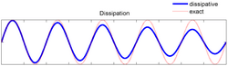
Figure 1: Figure 1: Illustration of pure numeric dissipation effect on a single sinusoid, as it propagates along the spatial domain. Both exact and simulated dissipative waves begin with the same amplitude; however, the amplitude of the dissipative wave decreases over time, but stays in phase.

Figure 2: Figure 2: Effect of numerical dissipation on a step function applied to the advection equation ut+ux=0 .
In a numerical scheme, a situation where waves of different frequencies are damped by different amounts, is called numerical dissipation, see figure (1). Generally, this results in the higher frequency components being damped more than lower frequency components. The effect of dissipation therefore is that sharp gradients, discontinuities or shocks in the solution tend to be smeared out, thus losing resolution, see figure (2). Fortunately, in recent years, various high resolution schemes have been developed to obviate this effect to enable shocks to be captured with a high degree of accuracy, albeit at the expense of complexity. Examples of particularly effective schemes are based upon flux/slope limiters [Wes-01] and WENO methods [Shu-98]. Dissipation can be introduced by numerical discretization of a partial differential equation that models a non-dissipative process. Generally, dissipation improves stability and, in some numerical schemes it is introduced deliberately to aid stability of the resulting solution. Dissipation, whether real or numerically induced, tend to cause waves to lose energy.
The dissipation error as a result of discretization can be determined by comparing the magnitude of the numeric amplification factor ∣∣Gnumeric∣∣, with the magnitude of the exact amplification factor ∣∣Gexact∣∣ , over one time step. The relative numerical diffusion error or relative numerical dissipation error compares real physical dissipation with the anomalous dissipation that results from numerical discretization. It can be defined as
εD=∣∣Gnumeric∣∣∣∣Gexact∣∣,(56)
and the total dissipation error resulting from n steps will be
εDtotal=(∣∣Gnumeric∣∣n−∣∣Gexact∣∣n)u0.(57)
If εD>1 for a given value of θ or Co, this discretization scheme will be unstable and a modification to the scheme will be necessary.
As mentioned above, if the imaginary part of ω(k) is zero for a particular discretization, then the scheme is non-dissipative.
Numerical dispersion

Figure 3: Figure 3: Illustration of pure numeric dispersion effect on a single sinusoid, as it propagates along the spatial domain. Both exact and simulated dispersive waves start in phase; however, the phase of the dispersive wave lags the exact wave over time, but its amplitude is unaffected.

Figure 4: Figure 4: Effect of numerical dispersion on a step function applied to the advection equation ut+ux=0 .
In a numerical scheme, a situation where waves of different frequencies move at different speeds without a change in amplitude, is called numerical dispersion – see figure (3). Alternatively, the Fourier components of a wave can be considered to disperse relative to each other. It therefore follows that the effect of a dispersive scheme on a wave composed of different harmonics, will be to deform the wave as it propagates. However the energy contained within the wave is not lost and travels with the group velocity. Generally, this results in higher frequency components traveling at slower speeds than the lower frequency components. The effect of dispersion therefore is that often spurious oscillations or wiggles occur in solutions with sharp gradient, discontinuity or shock effects, usually with high frequency oscillations trailing the particular effect, see figure (4). The degree of dispersion can be determined by comparing the phase of the numeric amplification factor ∣∣Gnumeric∣∣, with the phase of the exact amplification factor ∣∣Gexact∣∣ , over one time step. Dispersion represents phase shift and results from the imaginary part of the amplification factor. The relative numerical dispersion error compares real physical dispersion with the anomalous dispersion that results from numerical discretization. It can be defined as
εP=ΦnumericΦexact,(58)
where Φ=∠G=tan−1(Im{G}Re{G}) . The total phase error resulting from n steps will be
εPtotal=n(Φnumeric−Φexact)(59)
If εP>1 , this is termed a leading phase error. This means that the Fourier component of the solution has a wave speed greater than the exact solution. Similarly, if εP<1 , this is termed a lagging phase error. This means that the Fourier component of the solution has a wave speed less than the exact solution.
Again, high resolution schemes can all but eliminate this effect, but at the expense of complexity. Although many physical processes are modeled by PDE’s that are non-dispersive, when numerical discretization is applied to analyze them, some dispersion is usually introduced.
Group and phase velocity
The term group velocity refers to a wave packet consisting of a low frequency signal modulated (or multiplied) by a higher frequency wave. The result is a low frequency wave, consisting of a fundamental plus harmonics, that propagates with group velocity cg along a continuum oscillating at a higher frequency. Wave energy and information signals propagate at this velocity, which is defined as being equal to the derivative of the real part of the frequency ω , with respect to wavenumber k (scalar or vector proportional to the number of wave lengths per unit distance), i.e.
cg=dRe{ω(k)}dk.(60)
If there are a number of spatial dimensions then the group velocity is equal to the gradient of frequency with respect to the wavenumber vector, i.e. cg=∇Re{ω(k)} .
The complementary term to group velocity is phase velocity, cp , and this refers to the speed of propagation of an individual frequency component of the wave. It is defined as being equal to the real part of the ratio of frequency to wavenumber, i.e.
cp=Re{ωk}.(61)
It can also be viewed as the speed at which a particular phase of a wave propagates; for example, the speed of propagation of a wave crest. In one wave period T the crest advances one wave length λ ; therefore, the phase velocity is also given by cp=λ/T . We see that this second form is equal to equation (61) due to the following relationships: wavenumber k=2πλ and frequency ω=2πf where f=1T .
For a non-dispersive wave the phase error is zero and therefore cg=cp .
To calculate group and phase velocity for linear waves (or small amplitude waves) we assume a solution of the form u(x,t)=Aei(kx−ωt) , where A is a constant and x can be a scalar or vector, and substitute into the wave equation (or linearized wave equation) under consideration. For example, for ut+ux+uxxx=0 we obtain the dispersion relation ω=k−k3 , from which we calculate the group and phase velocities to be cg=1−3k2 and cp=1−k2 respectively. Thus, we observe that cg≠cp and that therefore, this example is dispersive.
Wellposedness
For most practical situations our interest is primarily in solving partial differential equations numerically; and, before we embark on implementing a numerical procedure, we would usually like to have some idea as to the expected behaviour of the system being modeled, ideally from an analytical solution. However, an analytical solution is not usually available; otherwise we would not need a numerical solution. Nevertheless, we can usually carry out some basic analysis that may give some idea as to steady state, long term trend, bounds on key variables, and reduced order solution for ideal or special conditions, etc. One key estimate that we would like to know is whether the fundamental system is stable or well posed. This is particularly important because if our numerical solution produces seemingly unstable results we need to know if this is fundamental to the problem or whether it has been introduced by the solution method we have selected to implement. For most situations involving simulation this is not a concern as we would be dealing with a well analyzed and documented system. But there are situations where real physical systems can be unstable and we need to know these in advance. For a real system to become unstable there needs to be some form of energy source: kinetic, potential, reaction, etc., so this can provide a clue as to whether or not the system is likely to become unstable. If it is, then we may need to modify our computational approach so that we capture the essential behaviour correctly – although a complete solution may not be possible.
In general, solutions to PDE problems are sought to solve a particular problem or to provide insight into a class of problems. To this end existence, uniqueness and stability of the solution are of vital importance [Zwi-97, chapter 10]. Whilst at this introductory level we must restrict our discussion, it is desirable to emphasize that for a solution of an evolutionary PDE (together with appropriate ICs and BCs) to be useful we require that:
- A unique solution must exist. The question as to whether or not a solution actually exists can be rather complex, and an answer can be sought for analytic PDEs by application of the Cauchy-Kowalewsky theorem [Cou-62, pp39-56].
- The solution must be numerically stable if we are to be able to predict its evolution over time. If the physical system is actually unstable, then prediction may not be possible.
- The solution must depend continuously on data such as boundary/initial conditions, forcing functions, domain geometry, etc.
If these conditions are full-filled, then the problem is said to be well posed, in the sense of Hadamard [Had-23]. Numerical schemes for particular PDE systems can be analyzed mathematically to determine if the solutions remain bounded. By invoking Parseval’s theorem of equality this analysis can be performed in the time domain or in the Fourier domain. A good introduction to this subject is given by LeVeque [Lev-07], and more advanced technical discussions can be found in the monographs by Tao [Tao-05] and Kreiss & Lorenz [Kre-04].
Characteristics
Characteristics are surfaces in the solution space of an evolutionary PDE problem that represent wave-fronts upon which information propagates. For example, consider the 1D advection equation problem
ut=cux,u(x,t=0)=u0,t≥0(62)
where the characteristics are given by dx/dt=c . For this problem the characteristics are straight lines in the xt-plane with slope 1/c and, along which, the dependent variable u is constant. The consequence of this is that the initial condition propagates from left to right at constant speed c . But, for other situations such as the inviscid Burgers equation problem,
ut=uux,u(x,t=0)=u0,t≥0,(63)
the propagation speed is not constant and the shape of the characteristics depend upon the initial conditions. If the initial condition is monotonically increasing with x , the characteristics will not overlap and the problem is well behaved. However, if the initial conditions are not monotonically increasing with x , at some time t>0 the characteristics will overlap and the solution will become multi-valued and a shock will develop. In this situation we can only find a weak solution (one where the problem is re-stated in integral form) by appealing to entropy considerations and the Rankine-Hugoniot jump condition. PDEs other than equations (62) and (63), such as those involving conservation laws, introduce additional complexity such as rarefaction or expansion waves. We will not discuss these aspects further here, and for additional discussion readers are referred to [Hir-90, chap. 16].
The method of characteristics
The method of characteristics (MOC) is a numerical method for solving evolutionary PDE problems by transforming them into a set of ODEs. The ODEs are solved along particular characteristics, using standard methods and the initial and boundary conditions of the problem. For more information refer to [Kno-00],[Ost-94],[Pol-07].
MOC is a quite general technique for solving PDE problems and has been particularly popular in the area of fluid dynamics for solving incompressible transient flow in pipelines. For an introduction refer to [Stre-97, chap. 12].
General topics
We conclude with a brief overview of some general aspects relating to linear and nonlinear waves.
Galilean invariance
Certain wave equations are Galilean invariant, i.e. the equation properties remain unchanged under a Galilean transformation. For example:
- A Galilean transformation for the linear wave equation (4) is
u~=Au(±λx+C1,±λt+C2),(64)
-
- where A , C1 , C2 and λ are arbitrary constants.
- A Galilean transformation for the nonlinear KdV equation (28) is
u~=u(x−6λt,t)−λ,(65)
-
- where λ is an arbitrary constant.
Other invariant transformations are possible for many linear and nonlinear wave equations, for example the Lorentz transformation applied to Maxwell’s equations, but these will not be discussed here.
Plane waves

Figure 5: Figure 5: Plane sinusoidal wave where its source is assumed to be at x=−∞ , and its fronts are advancing from right to left.
A Plane wave is considered to exist far from its source and any physical boundaries so, effectively, it is located within an infinite domain. Its position vector remains perpendicular to a given plane and satisfies the 1D wave equation
1c2∂2u∂t2=∂2u∂x2(66)
with a solution of the form
u=u0cos(ωt−kx+ϕ)(67)
where c=ωk represents propagation velocity and ϕ the phase of the wave. See figure (5).
Refraction and diffraction
Wave crests do not necessarily travel in a straight line as they proceed – this may be caused by refraction or diffraction.
Wave refraction is caused by segments of the wave moving at different speeds resulting from local changes in characteristic speed, usually due to a change in medium properties. Physically, the effect is that the overall direction of the wave changes, its wavelength either increases or decreases but its frequency remains unchanged. For example, in optics refraction is governed by Snell’s law and in shallow water waves by the depth of water.
Wave diffraction is the effect whereby the direction of a wave changes as it interacts with objects in its path. The effect is greatest when the size of the object causing the wave to diffract is similar to the wavelength.
Reflection
Reflection results from a change of wave direction following a collision with a reflective surface or domain boundary. A hard boundary is one that is fixed which causes the wave to be reflected with opposite polarity, e.g. u(x−vt)→−u(x+vt) . A soft boundary is one that changes on contact with the wave, which causes the wave to be reflected with the same polarity, e.g. u(x−vt)→u(x+vt) . If the propagating medium is not isotropic, i.e. it is not spatially uniform, then a partial reflection can result, with an attenuated original wave continuing to propagate. The polarity of the partial reflection will depend upon the characteristics of the medium.
Consider a travelling wave situation where the domain has a soft boundary with incident wave ϕI=Iexp(jωt−k1x) , reflected wave ϕR=Rexp(jωt+k1x) and transmitted wave ϕT=Texp(jωt−k2x) . In addition, for simplicity, consider the medium on both sides of the boundary to be isotropic and non-dispersive, which implies that all three waves will have the same frequency. From the conservation of energy law we have ϕI+ϕR=ϕT for all t , which implies I+R=T. Also, on differentiating with respect to x , we obtain −ik1I+ik1R=−ik2T . Thus, on rearranging we have
TI=2k1k1+k2,(68)
RI=k1−k2k1+k2.(69)
Equations (68) and (69) indicate that:
- the transmitted wave is always in-phase with the incident wave, i.e.synchronized (in-step with) and no phase-shift
- the reflected wave is only in-phase with the incident wave if k1>k2.
Also, because cg=cp=ωk, if k1>k2, then this implies that cg1<cg2, see section (Group and phase velocity).
We mention two other quantities
τ=∣∣∣TI∣∣∣,(70)
ρ=∣∣∣RI∣∣∣,(71)
the so-called coefficients of transmission and reflection respectively.
Resonance describes a situation where a system oscillates at one of its natural frequencies, usually when the amplitude increases as a result of energy being supplied by a perturbing force. A striking example of this phenomena is the failure of the mile-long Tacoma Narrows Suspension Bridge. On 7 November 1940 the structure collapsed due to a nonlinear wave that grew in magnitude as a result of excitation by a 42 mph wind. A video of this disaster is available on line at: archive.org . Another less dramatic example of resonance that most people have experienced is the effect of sound feedback from loudspeaker to microphone.
A more complex form of resonance is autoresonance, a nonlinear phase-locking phenomenon which occurs when a resonantly driven nonlinear system becomes phase-locked (synchronized or in-step) with a driving perturbation or wave.
Doppler effect
The Doppler effect (or Doppler shift) relates to the change in frequency and wavelength of waves emitted from a source as perceived by an observer, where the source and observer are moving at a speed relative to each other. At each moment of time the source will radiate a wave and an observer will experience the following effects:
- Wave source moving towards the observer – To the observer the moving source has the effect of compressing the emitted waves and the frequency is perceived to be higher than the source frequency. For example, a sound wave will have a higher pitch and the spectrum of a light wave will exhibit a blueshift.
- Wave source moving away from the observer – To the observer this time, the recessional velocity has the effect of expanding the emitted waves such that a sound wave will have a lower pitch and the spectrum of a light wave will exhibit a redshift.
Perhaps the most famous discovery involving the Doppler effect, is that made in 1929 by Edwin Hubble in connection with the Earth’s distance from receding galaxies: the redshift of light coming from distant galaxies is proportional to their distance. This is known as Hubble’s law.
Transverse and longitudinal waves
Transverse waves oscillate in the plane perpendicular to the direction of wave propagation. They include: seismic S (secondary) waves, and electromagnetic waves, E (electric field) and H (magnetic field), both of which oscillate perpendicularly to each other as well to the direction of propagation of energy. Light, an electromagnetic wave, can be polarized (oriented in a specific direction) by use of a polarizing filter.
Longitudinal waves oscillate along the direction of wave propagation. They include sound waves (pressure, particle displacement, or particle velocity propagated in an elastic medium) and seismic P (earthquake or explosion) waves.
Surface water waves however, are an example of waves that involve a combination of both longitudinal and transverse motion.
Traveling waves
Traveling-wave solutions [Pol-08], [Gri-11], by definition, are of the form
u(x,t)=U(z),z=kx−λt ;(72)
where λ/k plays the role of the wave propagation velocity (the value λ=0 corresponds to a stationary solution, and the value k=0 corresponds to a space-homogeneous solution).
Traveling-wave solutions are characterized by the fact that the profiles of these solutions at different time instants are obtained from one another by appropriate shifts (translations) along the x-axis. Consequently, a Cartesian coordinate system moving with a constant speed can be introduced in which the profile of the desired quantity is stationary. For λ>0 and k>0 , the wave described by equation (72) travels along the x-axis to the right (in the direction of increasing x).
The term traveling-wave solution is also used in situations where the variable t plays the role of a spatial coordinate, y .
Standing waves

Figure 6: Figure 6: A standing wave
ℜ(ϕ(x,t)) .
Standing waves’ occur when two traveling waves of equal amplitude and speed, but opposite direction, are superposed. The effect is that the wave amplitude varies with time but it does not move spatially. For example, consider two waves ϕ1(x,t)=Φ1expi(ωt−kx) and ϕ2(x,t)=Φ2expi(ωt+kx) , where ϕ1 moves to the right and ϕ2 moves to the left. By definition we have Φ2=Φ2 , and by simple algebraic manipulation we obtain
ϕ(x,t)=ϕ1(x,t)+ϕ2(x,t),
=Φ1[expi(ωt−kx)+expi(ωt+kx)],
⇓
=2Φ1expiωtcoskx.(73)
A standing wave is illustrated in figures (6) and (7) by a plot of the real part of equation (73), i.e. ℜ(ϕ(x,t))=2Φ1cosωtcoskx with k=1 , ω=1 and Φ1=12 .

Figure 7: Figure 7: Animated standing wave
ℜ(ϕ(x,t)) .
The points at which ϕ=0 are called nodes and the points at which ϕ=2∣∣Φ∣∣ are called antinodes. These points are fixed and occur at kx=(2n+1)π2 and kx=(2n+1)π respectively (n=±1,±2,⋯) .
Clearly, the existence of nonlinear standing waves can be demonstrated by application of Fourier analysis.
Waveguides
The idea of a waveguide is to constrain a wave such that its energy is directed along a specific path. The path may be fixed or capable of being varied to suit a particular application.
The operation of a waveguide is analyzed by solving the appropriate wave equation, subject to the prevailing boundary conditions. There will be multiple solutions, or modes, which are determined by the eigenfunctions associated with the particular wave equations, and the velocity of the wave as it propagates along the waveguide will be determined by the eigenvalues of the solution.
- An electromagnetic waveguide is a physical structure, such as a hollow metal tube, solid dielectric rod or co-axial cable that guides electromagnetic waves in the sub-optical (non-visible) electromagnetic spectrum
- An optical waveguide is a physical structure, such as an optical fiber, that guides waves in the optical (visible) part of the electromagnetic spectrum
- An acoustic waveguide is a physical structure, such as a hollow tube or duct (a speaking tube), that guides acoustic waves in the audible frequency range. Musical wind instruments, such as a flute, can also be thought of as acoustic waveguides.
For detailed analysis and further discussion refer to [Lio-03],[Oka-06].
Wave-front

Figure 8: Figure 8: Circular wave-fronts emanating from a point source.
As a wave propagates through a medium, the wavefront represents the outward normal surface formed by points in space, at a particular instant, as the wave travels outwards from its origin.
One of the simplest form of wavefront to envisage is an expanding circle where its radius r , expands with velocity v , i.e. r=vt. Simple circular sinusoidal wave-fronts propagating from a point source are shown in figure (8). They can be described by
u(r,t)=Re{exp[i(kr−ωt+π/2−ψ]},(74)
where k= wavenumber, r=radius , t=time , ω=frequency , ψ=phase angle .
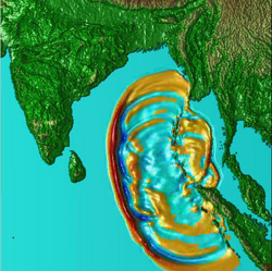
Figure 9: Figure 9: A snapshot from a simulation of the Indian Ocean tsunami that occurred on 26th December 2004 resulting from an earthquake off the west coast of Sumatra. The non-circular wave-fronts are clearly visible, which indicates curved rays. See animation here
.
Depending upon the particular wave equation and medium in which the wave travels, the wavefront may not appear to be an expanding circle. The path upon which any point on the wave front has traveled is called a ray, and this can be a straight line or, more likely, a curve in space. In general, the wavefront is perpendicular to the ray path, and the ray curvature will depend on the circumstances of the particular physical situation. For example, its curvature will be influenced by: an anisotropic medium, refraction, diffraction, etc.
Consider a water wave where wave height is very much smaller than water depth h . Its speed of propagation c , or celerity, is given by c=gh‾‾‾√ ; thus, for an ocean with varying depth the velocity will vary at different locations (refraction). This can result in waves having non-circular wave-fronts and hence curved rays. This situation, which occurs in many different applications, is illustrated in figure (9) where the curved wave-fronts are due to a combination of effects due to refraction, diffraction, reflection and a non-point disturbance.
Huygens’ principle

Figure 10: Figure 10: Advancing envelope of wave-fronts Φq0(t) .
We can consider all points of a wave-front of light in a vacuum or transparent medium to be new sources of wavelets that expand in every direction at a rate depending on their velocities.
This idea was originally proposed by the Dutch mathematician, physicist, and astronomer, Christiaan Huygens, in 1690, and is a powerful method for studying various optical phenomena [Enc-09]. Thus, the points on a wave can be viewed as each emitting a circular wave which combine to propagate the wave-front Φq0(t) . The wave-front can be thought of as an advancing line tangential to these circular waves – see figure (10). The points on a wave-front propagate from the wave source along so-called rays. The Huygens’ principle applies generally to wave-fronts and the laws of reflection and refraction can both be derived from Huygens’ principle. These results can also be obtained from Maxwell’s equations.
For detailed analysis and proof of Huygens’ principle, refer to [Arn-91].
There are an extremely large number of types and forms of shock wave phenomena, and the following are representative of some subject areas where shocks occur:
- Fluid mechanics: Shocks result when a disturbance is made to move through a fluid faster than the speed of sound (the celerity) of the medium. This can occur when a solid object is forced through a fluid, for example in supersonic flight. The effect is that the states of the fluid (velocity, pressure, density, temperature, entropy) exhibit a sudden transition, according to the appropriate conservation laws, in order to adjust locally to the disturbance. As the cause of the disturbance subsides, the shock wave energy is dissipated within the fluid and it reduces to a normal, subsonic, pressure wave. Note: A shock wave can result in local temperature increases of the fluid. This is a thermodynamic effect and should not be confused with heating due to friction.
- Mechanics: Bull whips can generate shocks as the oscillating wave progresses from the handle to the tip. This is because the whip is tapered from handle to the tip and, when cracked, conservation of energy dictates that the wave speed increases as it progresses along the flexible cord. As the wave speed increases it reaches a point where its velocity exceeds that of sound, and a sharp crack is heard.
- Continuum mechanics: Shocks result from a sudden impact, earthquake, or explosion.
- Detonation: Shocks result from an extremely fast exothermic reaction. The expansion of the fluid, due to temperature and chemical changes force fluid velocities to reach supersonic speed, e.g. detonation of an explosive material such as TNT. But perhaps the most striking example would be the shock wave produced by a thermonuclear explosion.
- Medical applications: A non-invasive treatment for kidney or gall bladder stones whereby they can be removed by use of a technique called extracorporeal lithotripsy. This procedure uses a focused, high-intensity, acoustic shock wave to shatter the stones to the point where they are reduced in size such that they may be passed through the body in a natural way!
For further discussion relating to shock phenomena see ([Ben-00],[Whi-99]).
We briefly introduce two topics below by way of example.
Blast Wave – Sedov-Taylor Detonation
A blast wave can be analyzed from the following equations,
∂ρ∂t+v∂ρ∂r+ρ(∂v∂r+2vr)=0,(75)
∂v∂t+v∂v∂r+1ρ∂p∂r=0,(76)
∂(p/ργ)∂t+v∂(p/ργ)∂r=0,(77)
where ρ , v , p , r , t and γ represent density of the medium in which the blast takes place (air), velocity of the blast front, blast pressure, blast radius, time and isentropic exponent (ratio of specific heats) of the medium respectively. Now, if we assume that,
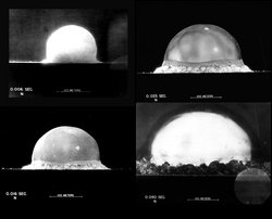
Figure 11: Figure 11: Time-lapse photographs with distance scales (100 m) of the first atomic bomb explosion in the New Mexico desert – 5.29 A.M. on 16th July, 1945. Times from instant of detonation are indicated in bottom left corner of each photograph (Top first – left column: 0.006s, 0.016s; right column: 0.025s, 0.09s).
- the blast can be considered to result from a point source of energy;
- the process is isentropic and the medium can be represented by the equation-of-state, (γ−1)e=p/ρ , where e represents internal energy;
- there is spherical symmetry;
then, after some analysis, similarity considerations lead to the following equation [Tay-50b]
E=cR5ρt2,(78)
where c is a similarity constant, R is the radius of the wave front and E is the total energy released by the explosion.
Back in 1945 Sir Geoffrey Ingram Taylor was asked by the British MAUD (Military Application of Uranium Detonation) Committee to deduce information regarding the power of the first atomic explosion in New Mexico. He derived this result, which was based on his earlier classified work [Tay-41], and was able to estimate, using only photographs of the blast (released into the public domain in 1947), that the yield of the bomb was equivalent to between 16.8 and 22.9 kilo-tons of TNT for values of γ equal to 1.4 and 1.3 respectively. Each of these photographs, crucially, contained a distance scale and precise time, see figure (11). Taylor used a value for the similarity constant of c=0.856 that he obtained by a step-by-step method. However the correct analytical value for this constant was later shown to be 0.8501 [Sed-59].
This result was classified secret but, five years later he published the details [Tay-50a],[Tay-50b], much to the consternation of the British government. J. von Neumann and L. I. Sedov published similar independently derived results [Bet-47],[Sed-46]. For further discussion relating to the theory refer to [Kam-00],[Deb-58].
Sonic boom

Figure 12: Figure 12: The N-wave sonic boom.
As an aircraft proceeds in smooth flight at a speed greater than the speed of sound – the sound barrier – a shock wave is formed at its nose and finishes at its tail. The speed of sound is given by c=γRT/MW‾‾‾‾‾‾‾‾‾√ , where γ , R , T and MW represent ratio of specific heats, universal gas constant, temperature and molecular weight respectively, and c≃330m/s at sea level for dry air at 0oC . The shock forms a high pressure, cone-shaped surface propagating with the aircraft. The half-angle (between direction of flight and the shock wave) θ is given by sin(θ)=1/M , where M=vaircraft/c is known as the Mach number of the aircraft. Clearly, as vaircraft increases, the cone becomes more pointed (θ becomes smaller).

Figure 13: Figure 13: The U-wave sonic boom.
As the aircraft continues under steady flight conditions at high speed, there will be an abrupt rise in pressure at the aircraft’s nose, which falls towards the tail when it then becomes negative. This is the so-called N-wave [Nak-08] – a pressure wave measured at sufficient distance such that it has lost its fine structure, see figure (12). A sonic boom occurs when the abrupt changes in pressure are of sufficient magnitude. Thus, steady supersonic flight results in two booms: one resulting from the rapid rise in pressure at the nose, and another when the pressure returns to normal as the tail passes the point vacated by the nose. This is the cause of the distinctive double boom from supersonic aircraft. At ground level typically, 10<Pmax<500Pa and τ≃0.001−0.005s. The duration T varies from around 100 ms for a fighter plane to 500 ms for the Space Shuttle or Concorde.

Figure 14: Figure 14:A USAF B1B makes a high speed pass at the Pensacola Beach airshow – Florida, July 12, 2002. Copyright © Gregg Stansbery, Stansbery Photography – reproduced with permission.
Another form of sonic boom is the focused boom. These can result from high speed aircraft flight maneuvering operations. These result in the so-called U-waves which have positive shocks at the front and rear of the boom, see figure (13). Generally, U-waves result in higher peak over-pressures than N-waves – typically between 2 and 5 times. At ground level typically, 20<Pmax<2500Pa (although they can be much higher). The highest overpressure ever recorded was 6800 Pa [144 lbs/sq-ft] (source: USAF Fact Sheet 96-03). For further discussion related to sonic booms refer to [Kao-04].
As an aircraft passes through, or close to the sound barrier, water vapor in the air is compressed by the shock wave and becomes visible as a large cloud of condensation droplets formed as the air cools due to low pressure at the tail. A smaller shock wave can also form on top of the canopy. This phenomena is illustrated in figure (14).
Solitary waves and solitons
The correct term for a wave which is localized and retains its form over a long period of time is: solitary wave. However, a soliton is a solitary wave having the additional property that other solitons can pass through it without changing its shape. But, in the literature it is customary to refer to the solitary wave as a soliton, although this is strictly incorrect [Tao-08].
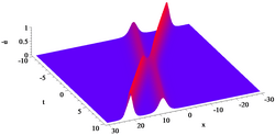
Figure 15: Figure 15: Evolution of a two-soliton solution of the KdV equation. Image illustrates the collision of two solitons that are both moving from left to right. The faster (taller) soliton overtakes the slower (shorter) soliton.
Solitons are stable, nonlinear pulses which exhibit a fine balance between non-linearity and dispersion. They often result from real physical phenomena that can be described by PDEs that are completely integrable, i.e. they can be solved exactly. Such PDEs describe: shallow water waves, nonlinear optics, electrical network pulses, and many other applications that arise in mathematical physics. Where multiple solitons moving at different velocities occur within the same domain, collisions can take place with the unexpected phenomenon that, first they combine, then the faster soliton emerges to proceed on its way. Both solitons then continue to proceed in the the same direction and eventually reach a situation where their speeds and shapes are unchanged. Thus, we have a situation where a faster soliton can overtake a slower soliton. There are two effects that distinguishes this phenomena from that which occurs in a linear wave system. The first is that the maximum height of the combined solitons is not equal to the sum of the individual soliton heights. The second is that, following the collision, there is a phase shift between the two solitons, i.e. the linear trajectory of each soliton before and after the collision is seen to be shifted horizontally – see figure (15).
Some additional discussion is given in section (The Korteweg-de Vries equation) and detailed technical overviews of the subject can be found in the works by Ablowitz & Clarkson [Abl-91], Drazin & Johnson [Dra-89] and Johnson [Joh-97]. Soliton theory is still an active area of research and a discussion on the various types of soliton solution that are known is given by Gerdjikov & Kaup [Ger-05].
Soliton types
Soliton types generally fall into thee types:
- Humps (pulses) – These are the classic bell-shaped curves that are typically associated with soliton phenomena.
- Kinks – These are solitons characterized by either a monotonic positive shift (kink) or a monotonic negative shift (anti-kink) where the change in value occurs gradually in the shape of an s-type curve.
- Breathers (bions) – These can be either stationary or travelling soliton humps that oscillate: becoming positive, negative, positive and so on.
More details may be found in Drazin and Johnson [Dra-89].
Tsunami
The word tsunami is a Japanese term derived from the characters 津 (tsu) meaning harbor and 波 (nami) meaning wave. It is now generally accepted by the international scientific community to describe a series of traveling waves in water produced by the displacement of the sea floor associated with submarine earthquakes, volcanic eruptions, or landslides. They are also known as tidal waves.
Tsunami are usually preceded by a leading-depression N-wave (LDN), one in which the trough reaches the shoreline first. Eyewitnesses in Banda Aceh who observed the effects of the December 2004 Sumatra Tsunami, see figure (9), resulting from a magnitude 9.3 seabed earthquake, described a series of three waves, beginning with a leading depression N wave [Bor-05]. Recent estimates indicate that this powerful tsunami resulted in excess of 275,000 deaths and extensive damage to property and infrastructure around the entire coast line of the Indian ocean [Kun-07].
Tsunami are long-wave phenomena and, because the wavelengths of tsunami in the ocean are long with respect to water depth, they can be considered shallow water waves. Thus, cp=cg=gh‾‾‾√ and for a depth of 4km we see that the wave velocity is around 200 m/s. Hence, tsunami waves are often modelled using the shallow water equations, the Boussinesq equation, or other suitable equations that bring out in sufficient detail the required wave characteristics. However, one of the major challenges is to model shoreline inundation realistically, i.e. the effect of the wave when it encounters the shore – also known as run-up. As the wave approaches the shoreline, the water depth decreases sharply resulting in a greatly increased surge of water at the point where the wave strikes land. This requires special modeling techniques to be used, such as robust Riemann solvers [Tor-01],[Ran-06] or the level-set method [Set-99],[Osh-03], which can handle situations where dry regions become flooded and vice versa.
Acknowledgements
The authors would like to thank reviewers Prof. Andrei Polyanin and Dr. Alexei Zhurov for their positive and constructive comments.
References
- [Abl-91] Ablowitz, M. J. and P. A. Clarkson (1991), Solitons, Nonlinear Evolution Equations and Inverse Scattering, London Mathematical Society lecture Notes 149, Cambridge University press.
- [Arn-91] Arnold, V. I. (1991), Mathematical Methods of Classical Mechanics, 2nd Ed., Springer.
- [Bar-03] Barenblatt, G. I. (2003), Scaling, Cambridge University Press.
- [Ben-00] Ben-Dor, G. (Ed), O. Igra (Ed) and T. Elperin (Ed) (2000), Handbook of Shock Waves, 3 vols, Academic Press.
- [Bet-47] Bethe, H. A., K. Fuchs, J.O. Hirschfelder, J. L. Magee, R. E. Peierls and J. von Neumann (1947), Blast Wave, Los Alamos Scientific Laboratory Report LA-2000.
- [Bor-05] Borrero, J. C. (2005). Field Data and Satellite Imagery of Tsunami Effects in Banda Aceh, Science 10 June, 308, p. 1596.
- [Buc-83] Buckley, R. (1985), Oscillations and Waves, Adam Hilger Ltd., Bristol and Boston.
- [Byn-84] Bynam, W. F., E. J. Browne and R. Porter Eds. (1984), Dictionary of The History of Science, Princton University Press.
- [Bur-93] Burden, R. L. and Faires, J. D. (1993), Numerical Analysis, 5th Ed., PWS Publishing Company.
- [Caj-61] Cajori, F. (1961), A History of Mathematics, MacMillan.
- [Cia-88] Ciarlet, P. G. (1988), Mathematical Elasticity: Three-dimensional Elasticity, volume 1, Elsevier.
- [Cla-89] Clarkson, P. A., A. S. Fokas and M. J. Ablowitz (1989), Hodograph transformations of linearizable partial differential equations, SIAM J. Appl. Mathematics, Vol. 49, No. 4, pp. 1188-1209.
- [Col-71] Collocott, T. C. (Ed.) (1971), Chambers Dictionary of Science and technology, Chambers.
- [Cor-05] Cornejo-Perez, O. and H. C. Rosu (2005), Nonlinear Second Order ODE’s: Factorizations And Particular Solutions, Progress of Theoretical Physics, 114-3, pp. 533-538.
- [Cou-62] Courant, R. and D. Hilbert (1962), Methods of Mathematical Physics – Vol II, Interscience Publishers.
- [Dai-06] Dai, H. H. , E. G. Fan and X. G. Geng (2006), Periodic wave solutions of nonlinear equations by Hirota’s bilinear method. Available on-line at: [1]
- [Deb-58] Deb Ray, G. (1958), An Exact Solution of a Spherical Blast Under Terrestrial Conditions, Proc. Natn. Inst. Sci. India, A 24, pp. 106-112.
- [Dis-08] DispersiveWiki (2008). An on-line collection of web pages concerned with the local and global well-posedness of various non-linear dispersive and wave equations. DispersiveWiki [2]
- [Dra-89] Drazin, P. G. and R. S. Johnson (1989), Solitons: an Introduction, Cambridge University press.
- [Elm-69] Elmore, W. C. and M. A. Heald (1969), Physics of Waves, Dover.
- [Enc-09] Encyclopædia Britannica (2009), Encyclopædia Britannica On-line, [3]
- [Far-93] Farlow, S. J. (1993), Partial Differential Equations for Scientists and Engineers, Chapter 17, Dover Publications, New York, New York.
- [Fow-05] Fowler, A. C. (2005), Techniques of Applied Mathematics, Report of the Mathematical Institute, Oxford University.
- [Gal-06] Galaktionov, V. A. and S. R. Svirshchevskii (2006), Exact Solutions and Invariant Subspaces of Nonlinear Partial Differential Equations in Mechanics and Physics, Chapman & Hall/CRC Press, Boca Raton.
- [Ger-05] Gerdjikov, V. S. and D. Kaup (2005), How many types of soliton solutions do we know? Seventh International Conference on Geometry, Integrability and Quantization, June 2-10, Varna, Bulgaria. I. M. Mladenov and M. De Leon, Editors. SOFTEX, Sofia 2005, pp. 1-24.
- [Gil-82] Gill, A. E. (1982), Atmosphere-Ocean Dynamics, Academic Press.
- [God-54] Godunov, S. K. (1954), Ph.D. Dissertation: Different Methods for Shock Waves, Moscow State University.
- [God-59] Godunov, S. K. (1959), A Difference Scheme for Numerical Solution of Discontinuous Solution of Hydrodynamic Equations, Math. Sbornik, 47, 271-306, translated US Joint Publ. Res. Service, JPRS 7226, 1969.
- [Gri-11] Griffiths, G. W. and W. E. Schiesser (2011), Traveling Wave Solutions of Partial Differential Equations: Numerical and Analytical Methods with Matlab and Maple, Academic Press; see also http://www.pdecomp.net/
- [Had-23]Hadamard, J. (1923), Lectures on Cauchy’s Problem in Linear Partial Differential Equations, Dover.
- [Ham-07] Hamdi, S., W. E. Schiesser and G. W. Griffiths (2007), Method of Lines. Scholarpedia, 2(7) 2859. Available on-line at Scholarpedia: [4]
- [He-06] He, J-H. and X-H. Wu (2006), Exp-function method for nonlinear wave equations, Chaos, Solitons & Fractals, Volume 30, Issue 3, November, pp. 700-708.
- [Her-05] Herman, W. and W. Malfliet (2005), The Tanh Method: A Tool to Solve Nonlinear Partial Differential Equations with Symbolic Software, 9th World Multiconference on Systemics, Cybernetics, and Informatics (WMSCI 2005), Orlando, Florida, July 10-13, pp. 165-168.
- [Hir-88] Hirsch, C. (1988), Numerical Computation of Internal and External Flows, Volume 1: Fundamentals of Numerical Discretization, Wiley.
- [Hir-90] Hirsch, C. (1990), Numerical Computation of Internal and External Flows, Volume 2: Computational Methods for Inviscid and Viscous Flows, Wiley.
- [Ibr-94] Ibragimov, N. H. (1994 – 1995), CRC Handbook of Lie Group Analysis of Differential Equations, Volumes 1 & 2, CRC Press, Boca Raton.
- [Inf-00] Infield, E. and G. Rowlands (2000). Nonlinear Waves, Solitons and Chaos, 2nd Ed., Cambridge University Press.
- [Jag-06] de Jager, E. M. (2006), On the Origin of the Korteweg-de Vries Equation, arXiv e-print service. Available on-line at: arXiv.org [5]
- [Joh-97] Johnson, R. S. (1999), A Modern Introduction to the Mathematical Theory of Water Waves, Cambridge University press.
- [Kao-04] Kaouri, K. (2004), PhD Thesis: Secondary Sonic Booms, Somerville College, Oxford University.
- [Kam-00] Kamm, J. R. (2000), Evaluation of the Sedov-von Neumann-Taylor Blast Wave Solution, Los Alamos National Laboratory Report LA-UR-00-6055.
- [Kar-98] Karigiannis, S. (1998). Minor Thesis: The inverse scattering transform and integrability of nonlinear evolution equations, University of Waterloo. Available on-line at: [6]
- [Kno-00] Knobel, R. A. (2000), An Introduction to the Mathematical Theory of Waves, American Mathematical Society.
- [Kor95] Korteweg, D. J. and de Vries, F. (1895), On the Change of Form of Long Waves Advancing in a Rectangular Canal, and on a New Type of Long Stationary Waves, Phil. Mag. 39, pp. 422-443.
- [Kre-04] Kreiss, H-O, and J. Lorenz (2004), Initial-Boundary Value problems and the Navier-Stokes Equations, Society for Industrial and Applied mathematics.
- [Krey-93]Kreyszig, E. (1993), Advanced Engineering Mathematics – Seventh Edition, Wiley.
- [Kun-07]Kundu, A. Ed. (2007), Tsunami and Nonlinear Waves, Springer.
- [Lam-93] Lamb, Sir H. (1993), Hydrodynamics, 6th Ed., Cambridge University Press.
- [Lan-98] Laney, Culbert B. (1998), Computational Gas Dynamics, Cambridge University Press.
- [Lev-02] LeVeque, R. J. (2002), Finite Volume Methods for Hyperbolic Problems, Cambridge University Press.
- [Lev-07] LeVeque, R. J. (2007), Finite Difference Methods for Ordinary and Partial Differential Equations, Society for Industrial and Applied mathematics.
- [Lig-78] Lighthill, Sir James (1978), Waves in Fluids, Cambridge University Press.
- [Lio-03] Lioubtchenko, D., S. Tretyakov and S. Dudorov (2003), Millimeter-wave Waveguides, Springer.
- [Mal-92] Mafliet, W. (1992), Solitary wave solutions of nonlinear wave equations, Am. J. Physics, 60(7), pp 650-654.
- [Mal-96a] Mafliet, W. and W. Hereman (1996a), The Tanh Method I – Exact Solutions of Nonlinear Evolution Wave Equations, Physica Scripta, 54, pp. 563-568.
- [Mal-96b] Mafliet, W. and W. Hereman (1996b), The Tanh Method II – Exact Solutions of Nonlinear Evolution Wave Equations, Physica Scripta, 54, pp. 569-575.
- [Mic-07] Microsoft Corporation (2007), Encarta® World English Dictionary [North American Edition], Bloomsbury Publishing Plc.
- [Mor-94] Morton, K. W. and D. F. Myers (1994), Numerical Solution of Partial Differential Equations, Cambridge.
- [Mur-02] Murray, J. D. (2002), Mathematical Biology I: An Introduction, 3rd Ed., Springer.
- [Mur-03] Murray, J. D. (2003), Mathematical Biology II: Spatial Models and Biomedical Applications, 3rd Ed., Springer.
- [Nak-08] Naka, Y., Y. Makino and T. Ito (2008). Experimental study on the effects of N-wave sonic-boom signatures on window vibration, pp 6085-90, Acoustics 08, Paris.
- [Oha-94] Ohanian, H. C. and R. Ruffini (1994), Gravitation and Spacetime, 2nd ed., Norton.
- [Oka-06] Okamoto, K. (2006), Fundamentals of Optical Waveguides, Academic Press.
- [Osh-03] Osher, S. and R. Fedkiw (2003). Level Set Methods and Dynamic Implicit Surfaces, Springer.
- [Ost-94] Ostaszewski, A. (1994), Advanced Mathematical Methods, Cambridge University press.
- [Pol-02] Polyanin, A. D., V. F. Zaitsev and A. Moussiaux (2002), Handbook of First Order Partial Differential Equations, Taylor & Francis.
- [Pol-04] Polyanin, A. D. and V. F. Zaitsev (2004), Handbook of Nonlinear Partial Differential Equations, Chapman and Hall/CRC Press.
- [Pol-07] Polyanin, A. D. and A. V. Manzhirov (2007), Handbook of Mathematics for Engineers and Scientists, Chapman and Hall/CRC Press.
- [Pol-08] Polyanin, A. D., W. E. Schiesser and A. I Zhurov (2008), Partial Differential Equation. Scholarpedia, 3(10):4605. Available on-line at Scholarpedia: [7]
- [Ran-06] Randall, D. L. and J. LeVeque (2006), Finite Volume Methods and Adaptive Refinement for Global Tsunami Propagation and Local Inundation, Science of Tsunami Hazards, 24(5), pp 319-328.
- [Ros-88] Ross, J., S. C. Muller, C. Vidal (1988), Chemical Waves, Science, 240, pp. 460-465.
- [Sch-94] Schiesser, W. E. (1994), Computational Mathematics in Engineering and Applied Science, CRC Press.
- [Sch-09] Schiesser, W. E. and G. W. Griffiths (2009), A Compendium of Partial Differential Equation Models: Method of Lines Analysis with Matlab, Cambridge University Press; see also http://www.pdecomp.net/
- [Sco-44] Scott-Russell, J. (1844), Report on Waves, 14th Meeting of the British Association for the Advancement of Science, pp. 311-390, London.
- [Sco-48] Scott-Russell, J. (1848), On Certain Effects Produced on Sound by The Rapid Motion of The Observer, 18th Meeting of the British Association for the Advancement of Science, pp. 37-38, London.
- [Sed-46] Sedov, L. I. (1946), Propagation of strong shock waves, Journal of Applied Mathematics and Mechanics, 10, pp241-250.
- [Sed-59] Sedov, L. I. (1959), Similarity and Dimensional Methods in Mechanics, Academic Press, New York.
- [Set-99] Sethian, J. A. (1999), Level Set methods and Fast Marching Methods, Cambridge University Press.
- [Sha-75] Shadowitz, A. (1975), The Electromagnetic Field, McGraw-Hill.
- [Shu-98] Shu, C-W. (1998), Essentially Non-oscillatory and Weighted Essential Non-oscillatory Schemes for Hyperbolic Conservation Laws. In: Cockburn, B., Johnson, C., Shu, C-W., Tadmor, E. (Eds.), Advanced Numerical Approximation of Nonlinear Hyperbolic Equations, Lecture Notes in Mathematics, vol 1697. Springer, pp. 325-432.
- [Shu-09] Shu, C-W. (2009), High Order Weighted Essentially Non-oscillatory Schemes for Convection Dominated Problems, SIAM Review, Vol. 51, No. 1, pp. 82-126.
- [Stra-92] Strauss, W. A. (1992), Partial Differential Equations: An Introduction, Wiley.
- [Stre-97] Streeter, V., K. W. Bedford and E. B. Wylie (1997), Fluid Mechanics, 9th Ed., McGraw-Hill.
- [Tan-97] Tannehill, J. C., et al. (1997), Computational Fluid Mechanics and Heat Transfer, 2nd Ed., Taylor and Francis.
- [Tao-05] Tao, T. (2005), Nonlinear dispersive equations: local and global analysis, Monograph based on (and greatly expanded from) a lecture series given at the NSF-CBMS regional conference on nonlinear and dispersive wave equations at New Mexico State University, held in June 2005. Available on-line at ucla.edu: [8]
- [Tao-08] Tao, T. (2008), Why are solitons stable?, arXiv:0802.2408v2 [math.AP]. Available on-line at arxiv.org: [9]
- [Tay-41] Taylor, Sir Geoffrey Ingram (1941), The formation of a blast wave by a very intense explosion, British Civil Defence Research Committee, Report RC-210.
- [Tay-50a] Taylor, Sir Geoffrey Ingram (1950), The Formation of a Blast Wave by a Very Intense Explosion. I. Theoretical Discussion, Proceedings of the Royal Society of London. Series A, Mathematical and Physical Sciences, Volume 201, Issue 1065, pp. 159-174.
- [Tay-50b] Taylor, Sir Geoffrey Ingram (1950), The Formation of a Blast Wave by a Very Intense Explosion. II. The Atomic Explosion of 1945, Proceedings of the Royal Society of London. Series A, Mathematical and Physical Sciences, Volume 201, Issue 1065, pp. 175-186.
- [Tor-99] Toro, E. F. (1999), Riemann Solvers and Numerical Methods for Fluid Dynamics, Springer-Verlag.
- [Tor-01] Toro, E. F. (2001), Shock-Capturing Methods for Free-Surface Shallow Flows, Wiley.
- [van-79] van Leer, B. (1979), Towards the ultimate conservative difference scheme V. A second order sequel to Godunov`s method, J. Comput. Phys., vol. 32, pp. 101-136.
- [Wes-01] Wesseling, P. (2001), Principles of Computational Fluid Dynamics, Springer, Berlin.
- [Whi-99] Whitham, G. B. (1999), Linear and Nonlinear Waves, Wiley.
- [Zie-77] Zienkiewicz, O. (1977) The Finite Element Method in Engineering Science. McGraw-Hill.
- [Zwi-97] Zwillinger, D. (1997), Handbook of Differential Equations, 3rd Ed., Academic Press.
Internal references
- Lawrence M. Ward (2008) Attention. Scholarpedia, 3(10):1538.
- Olaf Sporns (2007) Complexity. Scholarpedia, 2(10):1623.
- Tomasz Downarowicz (2007) Entropy. Scholarpedia, 2(11):3901.
- Jeff Moehlis, Kresimir Josic, Eric T. Shea-Brown (2006) Periodic orbit. Scholarpedia, 1(7):1358.
- Philip Holmes and Eric T. Shea-Brown (2006) Stability. Scholarpedia, 1(10):1838.


")


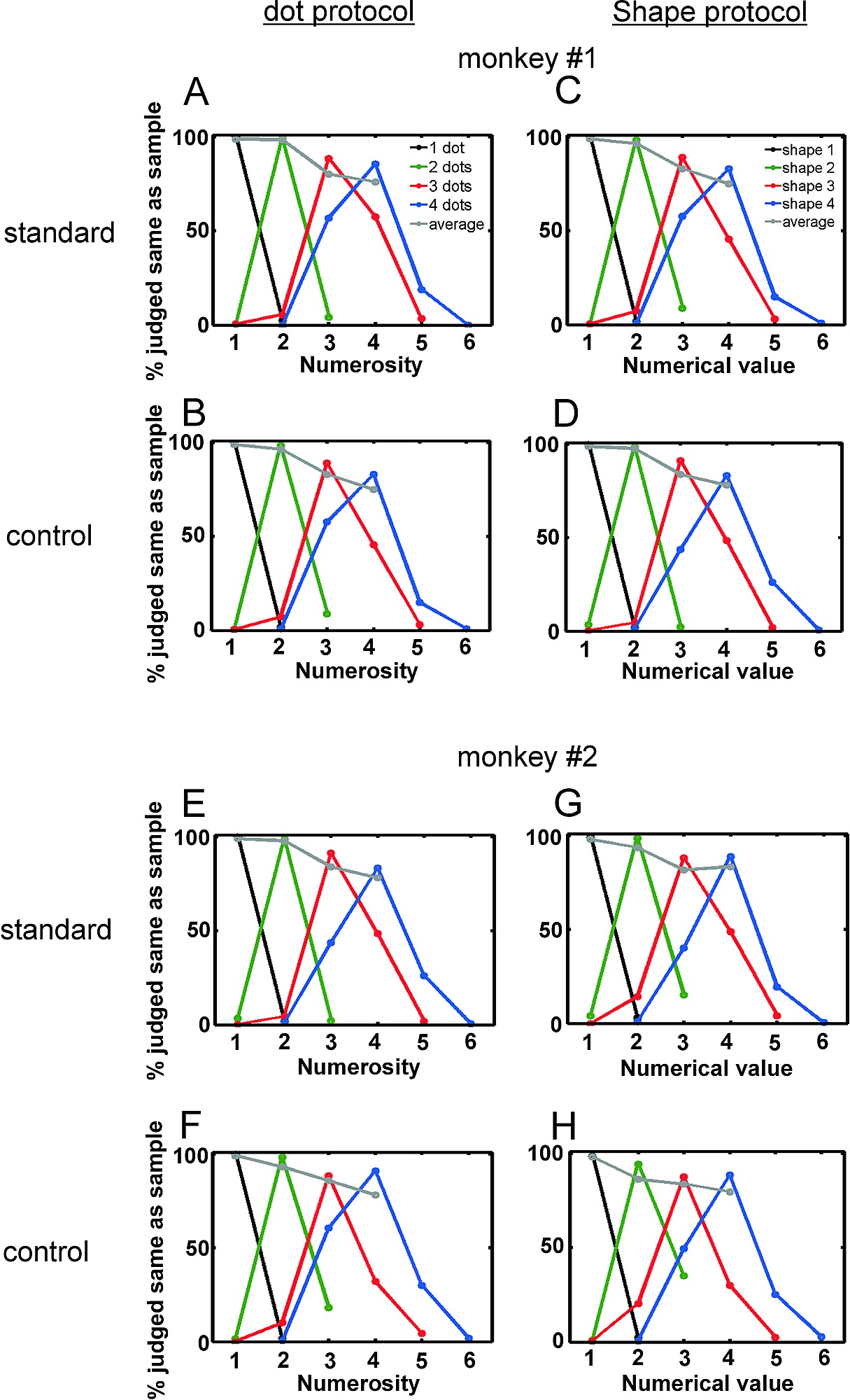


